

Excel’s conditional formatting feature allows users to visually highlight and analyze data based on specific criteria, making it easier to identify trends, patterns, and outliers at a glance. In this blog post, we will walk you through the steps to effectively use the Conditional Formatting Excel tool.
Step 1: Select the Data
Begin by selecting the range of cells that you want to apply conditional formatting to. You can click and drag to select multiple cells or use the shortcut key “Ctrl + Shift + Right Arrow” to select an entire column. For those working with Excel, conditional formatting is especially relevant when prepping data.
Step 2: Open the Conditional Formatting Menu
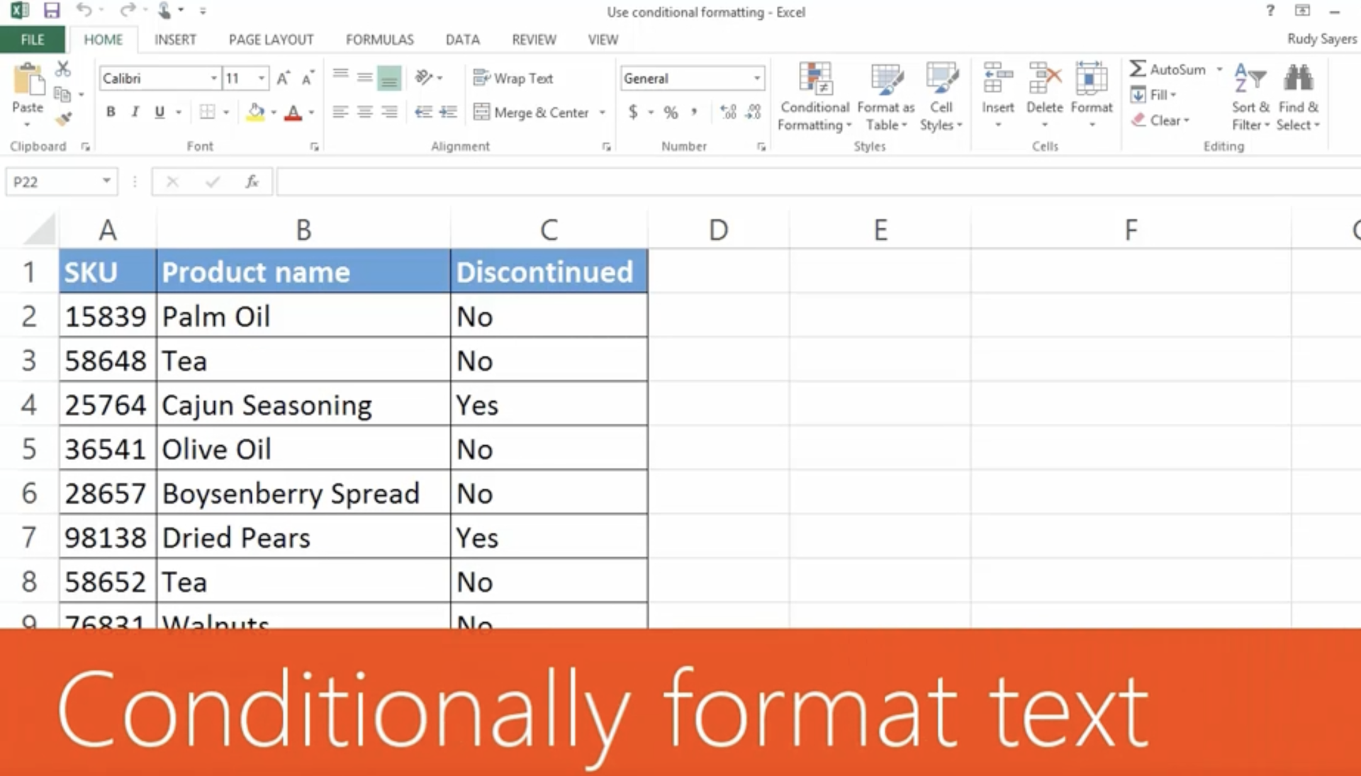
Go to the Home tab in the Excel ribbon and click on the “Conditional Formatting” button. A drop-down menu will appear with various formatting options. In Excel, the conditional formatting menus are central to applying dynamic visual changes.
Step 3: Choose a Conditional Formatting Rule
In the conditional formatting menu, you will see a list of predefined rules such as “Highlight Cell Rules,” “Top/Bottom Rules,” and “Data Bars.” When using Excel, these rules will guide you with conditional formatting for your specific needs.
- Highlight Cell Rules: This category includes rules like “Greater Than,” “Less Than,” “Between,” and “Equal To.” Select the rule that best fits your criteria, and a dialog box will appear where you can enter the specific values or formulas.
- Top/Bottom Rules: These rules allow you to highlight the top or bottom values in a selected range. You can choose to highlight the top or bottom percentage, number of items, or specific rank. Conditional Formatting in Excel lets you easily highlight these extreme values.
- Data Bars: Data bars provide a visual representation of the values in the selected range by adding a colored bar to each cell. The length of the bar corresponds to the value’s magnitude.
Step 4: Customize the Formatting
Once you’ve selected a rule, you can customize the formatting options to suit your needs. For example, you can choose a different highlight color, change the font style, or apply additional formatting, such as borders or font effects. With Excel’s conditional formatting features, customizing is quite flexible and powerful.
Step 5: Manage Conditional Formatting
If you need to make changes to your conditional formatting rules or want to apply multiple rules to the same range, you can manage your conditional formatting. To do this, go to the Home tab, click on the “Conditional Formatting” button, and select “Manage Rules” from the drop-down menu. It will open a dialogue box where you can modify or delete existing rules and add new ones. Conditional Formatting Excel provides easy-to-access tools for managing multiple formatting rules in your spreadsheet.
Step 6: Apply Conditional Formatting to Other Cells
If you want to apply the same conditional formatting rules to other cells or ranges, you can copy and paste the formatting. Select the cells with the desired formatting, press “Ctrl + C” to copy, then select the target cells where you want to apply the formatting. Right-click and choose “Paste Special,” and in the options, select “Formats.” This is a quick way to replicate your Conditional Formatting Excel settings across different areas of your worksheet.
Step 7: Clear Conditional Formatting
To remove conditional formatting from a specific range, select the cells and click on the “Conditional Formatting” button. In the drop-down menu, choose “Clear Rules” and select the appropriate option based on your requirements. It is important to clear Conditional Formatting rules in Excel when you want a fresh start for your data presentation.
By following these steps, you can effectively use conditional formatting in Excel to visually analyze your data with ease. This powerful feature enables you to gain insights and make informed decisions based on your data’s specific conditions. So, the next time you are working with large datasets, remember to use the Conditional Formatting options in Excel to enhance your analysis and presentation.